Lecture 4

Instruction Scheduling (part 3)

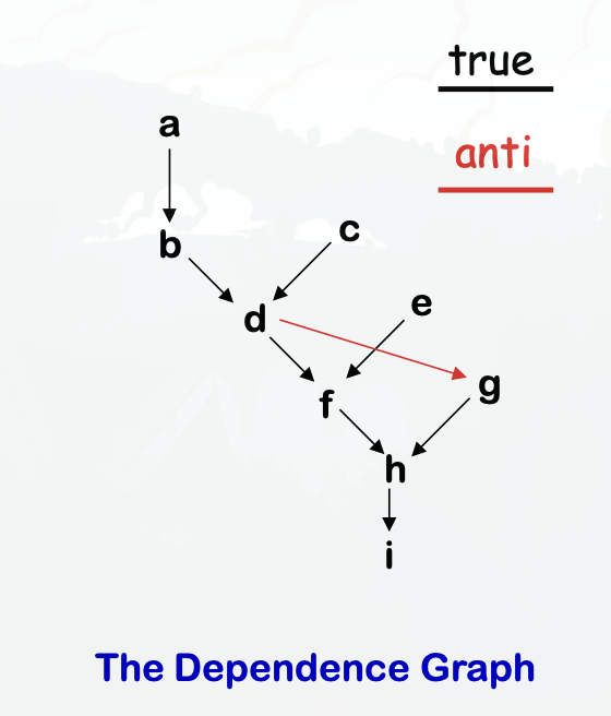
Code:

a:  loadAI  r0,@w   => r1
b:  add     r1,r1   => r1
c:  loadAI  r0,@x   => r2
d:  mult    r1,r2   => r1
e:  loadAI  r0,@y   => r3
f:  mult    r1,r3   => r1
g:  loadAI  r0,@z   => r2
h:  mult    r1,r2   => r1
i:  storeAI r1      => r0,@w

Note: store can cause aliasing issue, so for our projects we will always use storeAI

Local (forward) List Scheduling

Step 1. Build the dependence graph

Step 2. Determine priorities

Find the longest latency-weighted path

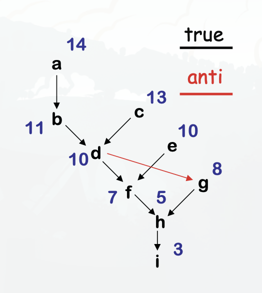
Example

You can schedule the instructions efficiently by prioritizing scheduling instructions in the critical path
Instructions that can be queued are stored in the Ready Set
Instructions that are currently queued are in the Active Set
You then traverse the graph, using the sets, and can generate more efficient, faster code.

Example:

Cycle	Ready Set	Active Set	What happened
	a, c, e		Move a to active set
0	c,e	a
1	e	a, c	Move c to active set
2		a, c, e	Move e to active set
3		b, c, e	Remove a from active set since it has finished, and add b to the ready set since it depended on a. Move b to active set
4		d, e	Remove b and c from active set since they have finished, and add d to the ready set since it depended on b. Move d to the active set
5		d	Remove e from the active set since it has finished. We can’t add f yet since it’s still waiting on d
6	f	g	Remove d form the active set, and add f and g to the ready set. We schedule g first because it has a higher latency-weighted path.
7		g, f	Move f to the active set
8		g, f	Nothing we can do here
9		h	Remove g and f from the active set since they have both finished. Add h to the ready set, and move it to the active set.
10		h	Nothing to do, waiting on h to finish
11			Remove h from the active set, and add i to the ready set. Move i to the active set
12			Nothing to do, waiting on i to finish

Generated Code

0:  a: loadAI r0,@w => r1
1:  c: loadAI r0,@x => r2
2:  e: loadAI r0,@y => r3
3:  b: add    r1,r1 => r1
4:  d: mult   r1,r2 => r1
5:
6:  g: loadAI r0,@z => r2
7:  f: mult   r1,r3 => r1
8:
9:  h: mult   r1,r2 => r1
10:
11: i: storeAI r1 => r0,@w
12:

By using the dependency graph and List scheduling, we turned 20 cycles into 14!

Algorithm

Cycle <- 0
Ready <- leaves of P
Active <- empty

while (Ready ∪ Active != empty)
  if (Ready != empty) then
    remove an op from Ready
    S(op) <- Cycle
    Active <- Active ∪ op

  Cycle <- Cycle + 1

  for each op ∈ Active
    if (S(op) + delay(op) <= Cycle) then
      remove op from Active
      for each successor s of op in P
        if (s is ready) then
          Ready <- Ready ∪ s

Formalisms

A correct schedule maps each n in N into a non-negative integer representing its cycle number such that

S(n) >= 0, for all n in N (obviously)
If (n1, n2) in E, S(n1) + delay(n1) <= S(n2)
For each type t, there are no more operations of type t in any cycle than the target machine can issue

The length of a schedule S, denoted L(S), is:

L(S) = max(n in N)(S(n) + delay(n))

The goal is to find the shortest possible correct schedule. S is time-optimal if L(S) <= L(S1), for all other schedules S1.

Note: We are trying to minimize execution time here.

What’s so difficult?

Critical points

All operands must be available
Multiple operations can be ready
Operands have multiple predecessors Together, these issues make scheduling hard (NP-Complete)

Local scheduling is the simple case

Restricted to straight-line code (single basic block)
Consistent and predictable latencies